Analyzing complex mixed-stock fisheries with 20 stocks
Sosthene Akia
Fisheries and Oceans Canadasosthene.akia@dfo-mpo.ca
Alex Hanke
Fisheries and Oceans Canadaalex.hanke@dfo-mpo.ca
2026-03-16
Source:vignettes/complex_mixed_stocks.Rmd
complex_mixed_stocks.RmdIntroduction
This tutorial demonstrates the capability of the RHISEA package to estimate stock proportions in complex mixed-stock fisheries involving 20 distinct source populations. It guides through generating simulated classification outputs (pseudo-classes, likelihoods, phi matrix), applying the five classical HISEA estimators, and visualizing the estimates.
Data Simulation of Classification Outputs
We simulate a mixture of 1000 fish from 20 stocks, generating pseudo-class assignments, likelihood matrices, and a phi matrix reflecting typical classification errors.
set.seed(1234)

np <- 20 # number of populations
n_mixture <- 1000

# Create stock names
stocks_names <- paste0("Stock_", seq_len(np))

# Simulate pseudo-classes randomly among stocks
pseudo_classes <- sample(seq_len(np), size = n_mixture, replace = TRUE)

# Simulate likelihood matrix: concentrated probabilities near true class + noise
likelihoods <- matrix(runif(n_mixture * np, min = 0.01, max = 0.05), nrow = n_mixture, ncol = np)
for (i in seq_len(n_mixture)) {
  likelihoods[i, pseudo_classes[i]] <- likelihoods[i, pseudo_classes[i]] + 0.8
}
# Normalize rows to sum to 1
likelihoods <- likelihoods / rowSums(likelihoods)

colnames(likelihoods) <- stocks_names

# Create a phi matrix with varying diagonal and asymmetric misclassification
base_correct <- runif(np, min = 0.5, max = 0.9)
phi_matrix <- matrix(0, nrow = np, ncol = np)
for (j in 1:np) {
  phi_matrix[j, j] <- base_correct[j]
  off_diag_total <- 1 - base_correct[j]
  off_diag_indices <- setdiff(1:np, j)
  off_diag_vals <- runif(length(off_diag_indices))
  off_diag_vals <- off_diag_vals / sum(off_diag_vals) * off_diag_total
  phi_matrix[off_diag_indices, j] <- off_diag_vals
}

colnames(phi_matrix) <- stocks_names
rownames(phi_matrix) <- stocks_names

# Check columns sum to 1 (optional)
round(colSums(phi_matrix), 6)
#>  Stock_1  Stock_2  Stock_3  Stock_4  Stock_5  Stock_6  Stock_7  Stock_8  Stock_9 Stock_10 Stock_11 Stock_12
#>        1        1        1        1        1        1        1        1        1        1        1        1
#> Stock_13 Stock_14 Stock_15 Stock_16 Stock_17 Stock_18 Stock_19 Stock_20
#>        1        1        1        1        1        1        1        1

# View phi_matrix with margins (optional)
addmargins(phi_matrix)
#>              Stock_1     Stock_2     Stock_3     Stock_4     Stock_5      Stock_6     Stock_7     Stock_8
#> Stock_1  0.500930313 0.029512468 0.006242553 0.028068041 0.040487460 0.0042663507 0.007404517 0.033587725
#> Stock_2  0.005900384 0.588945038 0.025207767 0.027255849 0.031520486 0.0045986343 0.031088868 0.041313159
#> Stock_3  0.011719231 0.032144016 0.563216021 0.028163042 0.022783123 0.0083950338 0.026835509 0.041142770
#> Stock_4  0.041678692 0.007713359 0.027489222 0.654983173 0.029357666 0.0065300549 0.007517548 0.014923598
#> Stock_5  0.042730290 0.015537590 0.036800452 0.004258260 0.537443926 0.0109881004 0.028955556 0.002942923
#> Stock_6  0.007163605 0.016743351 0.033839052 0.028027934 0.026312978 0.8703887497 0.007177561 0.033917636
#> Stock_7  0.026465621 0.037160276 0.005525758 0.018303780 0.031400284 0.0126300704 0.536204108 0.019026205
#> Stock_8  0.029929196 0.006553981 0.029791024 0.013319852 0.039610815 0.0091174242 0.038756926 0.515076716
#> Stock_9  0.054753345 0.044398838 0.003892038 0.006304059 0.027212499 0.0047196857 0.012452752 0.027923775
#> Stock_10 0.006850069 0.006288362 0.019349382 0.006324972 0.038465815 0.0015200206 0.008826723 0.001506658
#> Stock_11 0.054352542 0.003243054 0.016673950 0.029343436 0.020921000 0.0054286192 0.049960455 0.020628735
#> Stock_12 0.032109452 0.025054804 0.037704514 0.030868244 0.004259760 0.0056232391 0.054378328 0.041454764
#> Stock_13 0.027974795 0.021147707 0.012840866 0.002713035 0.023540078 0.0043011030 0.010247052 0.041154349
#> Stock_14 0.002650789 0.021110038 0.032015138 0.007389977 0.012451725 0.0076247329 0.034195994 0.042306726
#> Stock_15 0.001139765 0.028588886 0.017983176 0.031124399 0.037368423 0.0104681868 0.033306396 0.038445784
#> Stock_16 0.016301053 0.014461230 0.025195683 0.020590282 0.010688948 0.0125190960 0.027706525 0.001652608
#> Stock_17 0.032172241 0.015497043 0.039247368 0.019943631 0.001722050 0.0008158098 0.036061177 0.013532225
#> Stock_18 0.034834995 0.047259123 0.025728486 0.011030723 0.037869517 0.0016273769 0.028955626 0.002654864
#> Stock_19 0.028821500 0.029814472 0.008655597 0.028464826 0.020006399 0.0070184775 0.018371629 0.038611905
#> Stock_20 0.041522124 0.008826367 0.032601952 0.003522483 0.006577049 0.0114192344 0.001596751 0.028196876
#> Sum      1.000000000 1.000000000 1.000000000 1.000000000 1.000000000 1.0000000000 1.000000000 1.000000000
#>              Stock_9    Stock_10     Stock_11     Stock_12     Stock_13     Stock_14    Stock_15    Stock_16
#> Stock_1  0.029013471 0.020041898 7.307936e-04 0.0118828912 0.0131361367 0.0040295920 0.002077952 0.022830124
#> Stock_2  0.003029349 0.013165630 2.077272e-02 0.0083352660 0.0217304210 0.0057220405 0.012137826 0.019115478
#> Stock_3  0.018537045 0.020238823 4.345595e-03 0.0089143729 0.0411368250 0.0116009015 0.038897850 0.038276454
#> Stock_4  0.020231169 0.022432234 1.750497e-02 0.0096341175 0.0347490357 0.0155653603 0.039361042 0.025425551
#> Stock_5  0.006689371 0.021320576 2.231042e-02 0.0003671656 0.0079825165 0.0119364522 0.003883331 0.032472777
#> Stock_6  0.029319972 0.023989672 2.275309e-02 0.0118435261 0.0397261654 0.0132764887 0.042306448 0.014894133
#> Stock_7  0.027239313 0.003613266 1.933152e-02 0.0035704440 0.0434105844 0.0063101629 0.016865969 0.017977921
#> Stock_8  0.032026396 0.024705748 7.776468e-04 0.0067285752 0.0055067749 0.0111598572 0.008187408 0.020526667
#> Stock_9  0.654592196 0.019251316 5.963872e-03 0.0013553200 0.0032870170 0.0086037332 0.037698112 0.036810470
#> Stock_10 0.007239046 0.674025301 6.879909e-03 0.0038456978 0.0005928274 0.0082573875 0.011103948 0.001023450
#> Stock_11 0.001659935 0.015808447 7.975766e-01 0.0112899659 0.0248743503 0.0003489527 0.018746631 0.042751757
#> Stock_12 0.028499533 0.019511688 2.009561e-02 0.8651416419 0.0186654080 0.0155951664 0.001426930 0.038002436
#> Stock_13 0.011345108 0.023628600 1.024204e-05 0.0088638241 0.5999759634 0.0028782544 0.028991667 0.019010839
#> Stock_14 0.030759969 0.021401274 1.330992e-02 0.0112843045 0.0450071515 0.8243671152 0.009308273 0.002311103
#> Stock_15 0.003527243 0.002258160 5.604055e-03 0.0020858815 0.0390532193 0.0161618155 0.597105289 0.032615628
#> Stock_16 0.012447527 0.021247731 2.531701e-03 0.0028667696 0.0168204929 0.0062879510 0.028849773 0.533900041
#> Stock_17 0.029756704 0.011891996 2.147885e-04 0.0030714393 0.0240834099 0.0166669530 0.030513704 0.025014430
#> Stock_18 0.026843862 0.005269408 2.415207e-02 0.0074548494 0.0020948515 0.0018479216 0.003269296 0.037823509
#> Stock_19 0.018948778 0.020154022 1.094059e-02 0.0108027091 0.0131531680 0.0119645737 0.040487885 0.030939928
#> Stock_20 0.008294011 0.016044211 4.193878e-03 0.0106612384 0.0050136813 0.0074193204 0.028780666 0.008277305
#> Sum      1.000000000 1.000000000 1.000000e+00 1.0000000000 1.0000000000 1.0000000000 1.000000000 1.000000000
#>              Stock_17    Stock_18     Stock_19     Stock_20        Sum
#> Stock_1  9.333447e-03 0.007263802 0.0196557527 0.0547409215  0.8452362
#> Stock_2  2.494901e-02 0.011981678 0.0161434511 0.0233242709  0.9362373
#> Stock_3  8.365073e-03 0.010983623 0.0201768594 0.0371105318  0.9929827
#> Stock_4  2.283853e-02 0.015853941 0.0019665248 0.0351648259  1.0509206
#> Stock_5  2.031591e-02 0.018397569 0.0160155502 0.0144607085  0.8558094
#> Stock_6  1.150943e-02 0.013534077 0.0031730457 0.0453570624  1.2952540
#> Stock_7  2.138618e-02 0.020411420 0.0251982604 0.0306054577  0.9226366
#> Stock_8  3.935240e-03 0.007909484 0.0201376768 0.0019488405  0.8257062
#> Stock_9  1.205836e-02 0.020455378 0.0097399523 0.0401384293  1.0316112
#> Stock_10 3.277141e-05 0.005624286 0.0122498762 0.0401946218  0.8602011
#> Stock_11 9.900680e-03 0.021000367 0.0266943404 0.0239929512  1.1951968
#> Stock_12 2.537875e-02 0.001144115 0.0026868585 0.0276470495  1.2952483
#> Stock_13 2.156695e-02 0.012134468 0.0243822814 0.0010747547  0.8977819
#> Stock_14 1.242641e-02 0.017473556 0.0129170181 0.0305303978  1.1908416
#> Stock_15 2.526465e-02 0.005445251 0.0050968193 0.0232652831  0.9559083
#> Stock_16 6.767898e-03 0.023310920 0.0002548683 0.0109885435  0.7953896
#> Stock_17 7.349853e-01 0.014140439 0.0233795572 0.0123613648  1.0850717
#> Stock_18 3.057574e-03 0.747679555 0.0058795034 0.0001767373  1.0555098
#> Stock_19 5.322060e-03 0.012179845 0.7276984238 0.0141847469  1.0965415
#> Stock_20 2.060573e-02 0.013076224 0.0265533801 0.5327325010  0.8159150
#> Sum      1.000000e+00 1.000000000 1.0000000000 1.0000000000 20.0000000
Running Classic HISEA Estimators with
run_hisea_estimates()
Using the simulated classification outputs and phi matrix, we run all five classical estimators and summarize results.
results <- run_hisea_estimates(
  pseudo_classes = pseudo_classes,
  likelihoods = likelihoods,
  phi_matrix = phi_matrix,
  np = np,
  type = "BOOTSTRAP",
  stocks_names = stocks_names,
  export_csv = FALSE,
  verbose = TRUE
)
Displaying and Plotting Results
We print mean estimates by estimator and stock, and visualize estimated stock proportions.
print(results$mean_estimates)
#>               RAW       COOK      COOKC         EM         ML
#> Stock_1  0.052097 0.06635429 0.06635414 0.06635325 0.05305350
#> Stock_2  0.047889 0.04935680 0.04935666 0.04935643 0.04608110
#> Stock_3  0.048161 0.04214644 0.04214629 0.04214696 0.04765776
#> Stock_4  0.059126 0.05775113 0.05775098 0.05775087 0.06678241
#> Stock_5  0.040477 0.04496104 0.04496089 0.04496145 0.03264652
#> Stock_6  0.056068 0.03793922 0.03793907 0.03793919 0.06206818
#> Stock_7  0.045952 0.04844997 0.04844982 0.04844933 0.04316150
#> Stock_8  0.060229 0.08761090 0.08761075 0.08760981 0.06676397
#> Stock_9  0.042752 0.03074695 0.03074721 0.03074835 0.03838765
#> Stock_10 0.051352 0.06196865 0.06196850 0.06196840 0.05251769
#> Stock_11 0.047257 0.03104630 0.03104615 0.03104641 0.04556564
#> Stock_12 0.042142 0.02187131 0.02187372 0.02187402 0.03653358
#> Stock_13 0.044808 0.04616908 0.04616894 0.04616912 0.04119741
#> Stock_14 0.040807 0.02624482 0.02624468 0.02624475 0.03407448
#> Stock_15 0.064245 0.07549361 0.07549346 0.07549360 0.07688328
#> Stock_16 0.048778 0.06574371 0.06574356 0.06574283 0.04691440
#> Stock_17 0.050792 0.04388754 0.04388739 0.04388737 0.05064937
#> Stock_18 0.051985 0.04932299 0.04932284 0.04932299 0.05259370
#> Stock_19 0.052252 0.04283720 0.04283705 0.04283736 0.05209024
#> Stock_20 0.052831 0.07009805 0.07009790 0.07009751 0.05437762
print(results$sd_estimates)
#>                  RAW        COOK       COOKC          EM         ML
#> Stock_1  0.007154494 0.015060544 0.015060294 0.015058814 0.01251906
#> Stock_2  0.006829299 0.012021897 0.012022077 0.012021999 0.01189419
#> Stock_3  0.006428095 0.012029332 0.012029199 0.012027866 0.01132147
#> Stock_4  0.007445237 0.011774265 0.011774229 0.011774160 0.01295002
#> Stock_5  0.006400503 0.012335981 0.012335934 0.012335534 0.01100084
#> Stock_6  0.007446262 0.008871742 0.008871727 0.008871720 0.01314448
#> Stock_7  0.006543280 0.012696016 0.012695920 0.012695055 0.01139066
#> Stock_8  0.007536269 0.015218142 0.015218213 0.015218338 0.01316710
#> Stock_9  0.006245278 0.009929252 0.009928112 0.009926317 0.01093507
#> Stock_10 0.006893738 0.010486478 0.010486362 0.010486326 0.01204052
#> Stock_11 0.006596853 0.008669298 0.008669348 0.008669133 0.01146690
#> Stock_12 0.006327549 0.007617603 0.007610410 0.007609752 0.01096246
#> Stock_13 0.006620647 0.011390726 0.011390882 0.011390634 0.01163244
#> Stock_14 0.006168452 0.007739133 0.007739088 0.007739008 0.01092079
#> Stock_15 0.007835456 0.013659253 0.013659103 0.013659525 0.01380400
#> Stock_16 0.006722344 0.012923535 0.012923504 0.012923289 0.01160118
#> Stock_17 0.006974337 0.009753174 0.009753237 0.009753206 0.01204913
#> Stock_18 0.007003272 0.009651687 0.009651698 0.009651561 0.01215937
#> Stock_19 0.006925927 0.009838248 0.009838259 0.009838188 0.01193165
#> Stock_20 0.006887080 0.013459762 0.013459860 0.013459521 0.01195983

# Convert to tidy format for plotting
estimates_long <- as.data.frame(results$mean_estimates) %>%
  mutate(Stock = rownames(.)) %>%
  pivot_longer(-Stock, names_to = "Estimator", values_to = "Proportion")

ggplot(estimates_long, aes(x = Estimator, y = Proportion, fill = Stock)) +
  geom_bar(stat = "identity", position = position_dodge(width = 0.8)) +
  theme_minimal() +
  labs(
    title = "Estimated Stock Proportions by HISEA Estimator",
    y = "Estimated Proportion",
    x = "Estimator"
  ) +
  theme(axis.text.x = element_text(angle = 45, hjust = 1))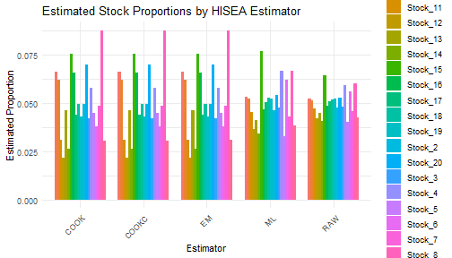
Conclusion
This tutorial illustrates that RHISEA is well suited for mixed-stock fisheries with numerous source populations. The simulation and estimation workflow scales to 20 stocks, producing robust and unbiased estimates using all classical HISEA estimators. This confirms the method’s applicability for complex, high-dimensional stock composition problems.