Verifying compatibility: RHISEA (R) vs FORTRAN HISEA

Introduction

This vignette demonstrates a full workflow to:

Load baseline and mixture data from package inst/extdata/
Simulate multiple datasets mimicking mixed-stock fishery data
Run HISEA estimators in R (run_hisea_all with LDA and LDA_MASS methods)
Run the Fortran executable (assumed available as hisea.exe) for comparison
Aggregate and visualize estimator results (R vs Fortran)
Export results to Excel
Perform simple diagnostics to detect large discrepancies between methods

1. Load baseline and mixture data from installed package

We store data in inst/extdata/ to ensure users can reproduce the analysis after installation.

baseline_file <- system.file("extdata", "baseline.rda", package = "RHISEA")
mixture_file  <- system.file("extdata", "mixture.rda",  package = "RHISEA")

load(baseline_file)  # loads `baseline` data.frame
load(mixture_file)   # loads `mixture` data.frame

# Convert baseline and mixture into HISEA file formats (.std and .mix)
write_std_from_dataframe(df=baseline, stock_col = "population", var_cols = c("d13c", "d18o"))
write_mix_from_dataframe(df=mixture, var_cols = c("d13c_ukn", "d18o_ukn"))

2. Define global parameters for simulation and analysis

np <- 2     # Number of populations (stocks)
nv <- 2     # Number of isotopic variables
Nsamps <- 1000  # Number of baseline resamples per simulation
Nmix <- 100     # Number of mixture individuals per simulation
stock_labels <- c("East", "West")
resample_baseline <- FALSE
resampled_baseline_sizes <- c(50, 50)
baseline_std_file <- "hisea.std"
mixture_mix_file <- "hisea.mix"

3. Utility functions for reading/writing HISEA files and Fortran outputs

# Read baseline and mixture files, split by stocks
read_base_std_mix <- function(std_path, mix_path) {
  std_lines <- readLines(std_path)
  mix_lines <- readLines(mix_path)
  split_index <- which(grepl("NEXT STOCK", std_lines, ignore.case = TRUE))
  end_std <- which(grepl("End of baseline data", std_lines, ignore.case = TRUE))
  stock1_base <- std_lines[1:(split_index - 1)]
  stock2_base <- std_lines[(split_index + 1):(end_std - 1)]
  end_mix <- which(grepl("End of mixed sample", mix_lines, ignore.case = TRUE))
  mix_base <- mix_lines[1:(end_mix - 1)]
  list(stock1 = stock1_base, stock2 = stock2_base, mix = mix_base)
}

# Write baseline (.std) file from list of matrices
write_std <- function(filepath, stock_list) {
  con <- file(filepath, "w")
  for (i in seq_along(stock_list)) {
    apply(stock_list[[i]], 1, function(row) writeLines(paste(row, collapse = " "), con))
    if (i < length(stock_list)) writeLines("NEXT STOCK", con)
  }
  writeLines("End of baseline data", con)
  writeLines("End of file", con)
  close(con)
}

# Write mixture (.mix) file from matrix
write_mix <- function(filepath, data) {
  con <- file(filepath, "w")
  apply(data, 1, function(row) writeLines(paste(row, collapse = " "), con))
  writeLines("End of mixed sample", con)
  writeLines("End of file", con)
  close(con)
}

# Read estimator results from Fortran output files, returns numeric vector of length 2 or NA
read_fort_estimator <- function(file_path) {
  if (!file.exists(file_path)) return(c(NA, NA))
  line <- readLines(file_path, warn = FALSE)[1]
  vals <- as.numeric(unlist(strsplit(trimws(line), "\\s+")))
  if (length(vals) == 2) return(vals) else return(c(NA, NA))
}

# Generate Poisson distributed baseline stock data for simulation
generate_stock_data <- function(n, n_vars, base_lambda_val) {
  if (base_lambda_val <= 0) base_lambda_val <- 0.1
  matrix(rpois(n * n_vars, lambda = base_lambda_val), ncol = n_vars)
}

4. Simulation setup and results containers

We simulate 50 datasets, run R estimators and Fortran executable, then store results.

# For reproducible parallel RNG streams
RNGkind("L'Ecuyer-CMRG")
set.seed(42)
n_sim <- 50

results <- list()     # R LDA results
results2 <- list()    # R LDA_MASS results
est_wide_comparisons <- vector("list", 5)  # 5 estimators to compare
est_long_comparisons <- vector("list", 5)

for (j in 1:5) {
  est_wide_comparisons[[j]] <- data.frame()
  est_long_comparisons[[j]] <- data.frame()
}

# Precompute RNG streams for independent simulations
streams <- vector("list", n_sim)
streams[[1]] <- .Random.seed
for (i in 2:n_sim) {
  streams[[i]] <- parallel::nextRNGStream(streams[[i - 1]])
}

5. Main simulation loop

for (i in 1:n_sim) {
  cat("\n--- Simulation ", i, " ---\n")

  # Activate independent RNG stream for reproducibility
  .Random.seed <- streams[[i]]

  # Simulate baseline stock data with slightly different lambda values per stock
  base_lambda_stock1 <- runif(1, 15, 25)
  lambda_shift_stock2 <- runif(1, 5, 15)
  stock1_data <- generate_stock_data(100, nv, base_lambda_stock1)
  stock2_data <- generate_stock_data(100, nv, base_lambda_stock1 + lambda_shift_stock2)

  # Write baseline to .std file
  write_std(baseline_std_file, list(stock1_data, stock2_data))

  # Generate mixture based on random proportions
  current_sim_comp <- as.numeric(gtools::rdirichlet(1, alpha = rep(1, np)))
  n_from_stocks <- round(Nmix * current_sim_comp)
  if (sum(n_from_stocks) != Nmix) n_from_stocks[1] <- n_from_stocks[1] + (Nmix - sum(n_from_stocks))

  mixture_data <- rbind(
    stock1_data[sample(nrow(stock1_data), n_from_stocks[1], replace = TRUE), ],
    stock2_data[sample(nrow(stock2_data), n_from_stocks[2], replace = TRUE), ]
  )
  mixture_data <- mixture_data[sample(nrow(mixture_data)), ]

  # Write mixture to .mix file
  write_mix(mixture_mix_file, mixture_data)

  # Run Fortran HISEA executable
  system("hisea.exe", wait = TRUE)
  out_file <- sprintf("hisea%02d.out", i)
  if (file.exists("hisea.out")) file.rename("hisea.out", out_file)

  # Run R-based estimations with LDA and LDA_MASS
  r_result <- run_hisea_all(
    type = "ANALYSIS",
    np = np,
    phi_method = "standard",
    nv = nv,
    resample_baseline = resample_baseline,
    resampled_baseline_sizes = resampled_baseline_sizes,
    seed_val = 123456,
    nsamps = Nsamps,
    Nmix = Nmix,
    baseline_input = baseline_std_file,
    mix_input = mixture_mix_file,
    method_class = "LDA",
    stocks_names = stock_labels
  )
  r_df <- as.data.frame(r_result$mean)
  colnames(r_df) <- paste0("Estimator_", 1:5)
  r_df$Stock <- stock_labels
  r_df$Simulation <- paste0("Sim_", i)
  results[[i]] <- r_df

  r_result2 <- run_hisea_all(
    type = "ANALYSIS",
    np = np,
    phi_method = "standard",
    nv = nv,
    resample_baseline = resample_baseline,
    resampled_baseline_sizes = resampled_baseline_sizes,
    seed_val = 123456,
    nsamps = Nsamps,
    Nmix = Nmix,
    baseline_input = baseline_std_file,
    mix_input = mixture_mix_file,
    method_class = "LDA_MASS",
    stocks_names = stock_labels
  )
  r_df2 <- as.data.frame(r_result2$mean)
  colnames(r_df2) <- paste0("Estimator_", 1:5)
  r_df2$Stock <- stock_labels
  r_df2$Simulation <- paste0("Sim_", i)
  results2[[i]] <- r_df2

  # Read Fortran estimators from fort.xx files (10 + estimator index)
  fort_estimates <- lapply(1:5, function(j) read_fort_estimator(sprintf("fort.%02d", 10 + j)))

  # Store wide and long format comparisons for each estimator
  for (j in 1:5) {
    wide_df <- data.frame(
      Simulation = paste0("Sim_", i),
      Stock = stock_labels,
      R = r_df[[paste0("Estimator_", j)]],
      Mass = r_df2[[paste0("Estimator_", j)]],
      Fortran = fort_estimates[[j]]
    )
    est_wide_comparisons[[j]] <- rbind(est_wide_comparisons[[j]], wide_df)

    long_df <- data.frame(
      Simulation = rep(paste0("Sim_", i), times = 6),
      Estimate = paste0("Estimator_", j),
      Stock = rep(stock_labels, times = 3),
      Method = rep(c("Fortran", "LDA_R", "LDA_MASS"), each = 2),
      Value = c(
        fort_estimates[[j]],
        r_df[[paste0("Estimator_", j)]],
        r_df2[[paste0("Estimator_", j)]]
      )
    )
    est_long_comparisons[[j]] <- rbind(est_long_comparisons[[j]], long_df)
  }
}
#> 
#> --- Simulation  1  ---
#> 
#> --- Simulation  2  ---
#> 
#> --- Simulation  3  ---
#> 
#> --- Simulation  4  ---
#> 
#> --- Simulation  5  ---
#> 
#> --- Simulation  6  ---
#> 
#> --- Simulation  7  ---
#> 
#> --- Simulation  8  ---
#> 
#> --- Simulation  9  ---
#> 
#> --- Simulation  10  ---
#> 
#> --- Simulation  11  ---
#> 
#> --- Simulation  12  ---
#> 
#> --- Simulation  13  ---
#> 
#> --- Simulation  14  ---
#> 
#> --- Simulation  15  ---
#> 
#> --- Simulation  16  ---
#> 
#> --- Simulation  17  ---
#> 
#> --- Simulation  18  ---
#> 
#> --- Simulation  19  ---
#> 
#> --- Simulation  20  ---
#> 
#> --- Simulation  21  ---
#> 
#> --- Simulation  22  ---
#> 
#> --- Simulation  23  ---
#> 
#> --- Simulation  24  ---
#> 
#> --- Simulation  25  ---
#> 
#> --- Simulation  26  ---
#> 
#> --- Simulation  27  ---
#> 
#> --- Simulation  28  ---
#> 
#> --- Simulation  29  ---
#> 
#> --- Simulation  30  ---
#> 
#> --- Simulation  31  ---
#> 
#> --- Simulation  32  ---
#> 
#> --- Simulation  33  ---
#> 
#> --- Simulation  34  ---
#> 
#> --- Simulation  35  ---
#> 
#> --- Simulation  36  ---
#> 
#> --- Simulation  37  ---
#> 
#> --- Simulation  38  ---
#> 
#> --- Simulation  39  ---
#> 
#> --- Simulation  40  ---
#> 
#> --- Simulation  41  ---
#> 
#> --- Simulation  42  ---
#> 
#> --- Simulation  43  ---
#> 
#> --- Simulation  44  ---
#> 
#> --- Simulation  45  ---
#> 
#> --- Simulation  46  ---
#> 
#> --- Simulation  47  ---
#> 
#> --- Simulation  48  ---
#> 
#> --- Simulation  49  ---
#> 
#> --- Simulation  50  ---

6. Aggregate and summarize results

final_results <- do.call(rbind, results)

# Round values and compute residuals between R and Fortran
for (j in 1:5) {
  est_wide_comparisons[[j]]$R <- round(est_wide_comparisons[[j]]$R, 4)
  est_wide_comparisons[[j]]$Mass <- round(est_wide_comparisons[[j]]$Mass, 4)
  est_wide_comparisons[[j]]$res <- est_wide_comparisons[[j]]$R - est_wide_comparisons[[j]]$Fortran
  est_wide_comparisons[[j]]$res_mass <- est_wide_comparisons[[j]]$Mass - est_wide_comparisons[[j]]$Fortran
}

7. Export results to Excel

write_xlsx(list(
  R_Only_Results = final_results,
  Estimator1_Comparison = est_wide_comparisons[[1]],
  Estimator2_Comparison = est_wide_comparisons[[2]],
  Estimator3_Comparison = est_wide_comparisons[[3]],
  Estimator4_Comparison = est_wide_comparisons[[4]],
  Estimator5_Comparison = est_wide_comparisons[[5]]
), path = "hisea_r_vs_fortran_results.xlsx")

cat("\nResults saved to hisea_r_vs_fortran_results.xlsx\n")
#> 
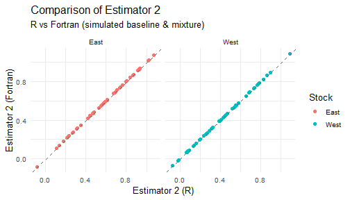
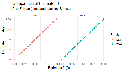
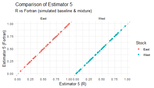
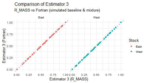
#> Results saved to hisea_r_vs_fortran_results.xlsx

8. Visualization: Compare R vs Fortran estimators

plot_estimator <- function(df, est_label) {
  ggplot(df, aes(x = R, y = Fortran, color = Stock)) +
    geom_point(size = 2) +
    facet_wrap(~Stock) +
    geom_abline(slope = 1, intercept = 0, linetype = "dashed", color = "gray40") +
    labs(
      title = paste("Comparison of", est_label),
      subtitle = "R vs Fortran (simulated baseline & mixture)",
      x = paste(est_label, "(R)"),
      y = paste(est_label, "(Fortran)")
    ) +
    theme_minimal(base_size = 13)
}

for (j in 1:5) {
  print(plot_estimator(est_wide_comparisons[[j]], paste0("Estimator ", j)))
}

Comparison of R vs Fortran estimates for each estimator

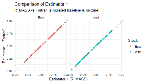
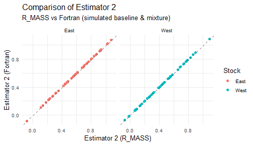
9. Visualization: Compare R_MASS vs Fortran estimators

plot_estimator2 <- function(df, est_label) {
  ggplot(df, aes(x = Mass, y = Fortran, color = Stock)) +
    geom_point(size = 2) +
    facet_wrap(~Stock) +
    geom_abline(slope = 1, intercept = 0, linetype = "dashed", color = "gray40") +
    labs(
      title = paste("Comparison of", est_label),
      subtitle = "R_MASS vs Fortran (simulated baseline & mixture)",
      x = paste(est_label, "(R_MASS)"),
      y = paste(est_label, "(Fortran)")
    ) +
    theme_minimal(base_size = 13)
}

for (j in 1:5) {
  print(plot_estimator2(est_wide_comparisons[[j]], paste0("Estimator ", j)))
}

Comparison of R_MASS vs Fortran estimates for each estimator

10. Boxplot for all estimators and methods

all_wide <- do.call(rbind, est_wide_comparisons)
all_long <- do.call(rbind, est_long_comparisons)

ggplot(all_long, aes(x = Method, y = Value, fill = Method)) +
  geom_point(position = position_jitter(width = 0.15), outlier.shape = NA) +
  stat_summary(
    fun = mean,
    geom = "point",
    shape = 23, size = 3,
    fill = "white"
  ) +
  stat_summary(
    fun = mean,
    geom = "text",
    aes(label = sprintf("%.4f", after_stat(y))),
    hjust = 1.2,
    vjust = 0.1,
    size = 3
  ) +
  facet_grid(Estimate ~ Stock) +
  theme_minimal() +
  labs(
    title = "Comparison of Estimation Methods Across Simulations",
    y = "Estimated Proportion",
    x = "Method"
  ) +
  theme(axis.text.x = element_text(angle = 45, hjust = 1))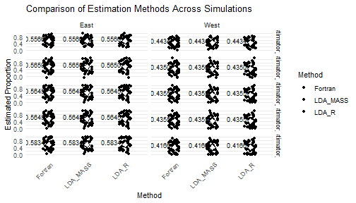

Boxplot comparing all methods across simulations

11. Diagnostics: Alert if large divergence detected

threshold <- 0.05  # 5% difference threshold
max_diffs <- sapply(est_wide_comparisons, function(df) max(abs(df$R - df$Fortran), na.rm = TRUE))

if (any(max_diffs > threshold)) {
  warning(
    paste(
      "Warning: Large divergence detected between R and Fortran estimators.",
      "Maximum differences by estimator:",
      paste0("Estimator", 1:5, "=", round(max_diffs, 3), collapse = "; ")
    )
  )
} else {
  message("No large divergences detected between R and Fortran estimators.")
}

Conclusion

This vignette provides a full workflow to simulate, run, compare and diagnose the HISEA estimation methods in R versus the original Fortran implementation. All results and plots help verify the consistency and quality of the R implementation, and the diagnostics alert when large discrepancies occur.

Sosthene Akia

Alex Hanke

2025-08-19